Beware of Probe Loading Artifacts with
Passive Probes
Passive probes are standard with most oscilloscopes, and jumper wires are often used to reach test points.
This article explores the hidden effects of probe loading —
and why the waveform you see may not reflect the true circuit signal.
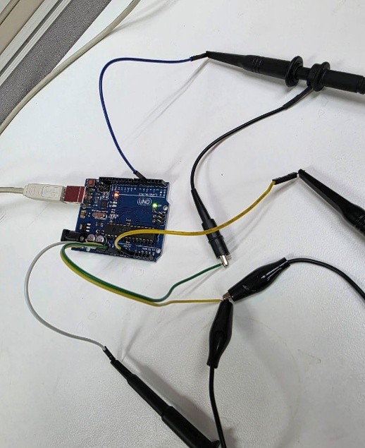
Fig 1 — Typical setup: jumper wires connect a passive probe to active electronics.
On an oscilloscope, a waveform like Fig 2 often appears — a “square” signal with overshoot, undershoot, and ringing.
Amplitude and frequency seem clear, leading many to assume this is the actual circuit signal. But is it?
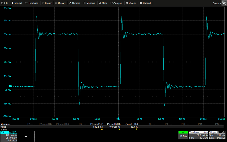
Fig 2 — Digital waveform captured with a passive probe. Note overshoot, undershoot, and ringing.
Setting up a Reference
A signal source is connected to oscilloscope channel 4 (C4) using coaxial cables with 50 Ω coupling.
The waveform is saved as M4 — our golden reference trace.
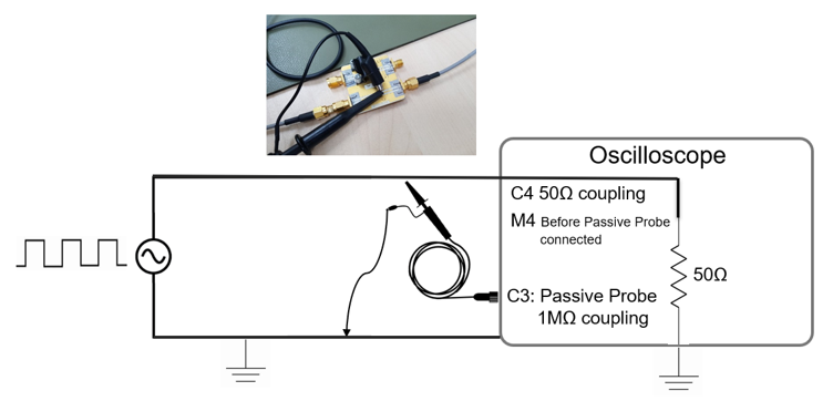
Fig 3 — Signal source connected to C4 at 50 Ω. A passive probe on C3 then probes the same path.
With M4 saved, a passive probe on channel 3 (C3) measures the same path. M4, C4, and C3 are displayed together (Fig 4) for comparison.
What the Data Reveals
Overshoot & undershoot up to 33%
Artefacts appear via passive probe — absent in the actual circuit.
Transition times overestimated by 50%
Rise/fall times are inflated, skewing timing analysis.
Amplitude & frequency remain accurate
Parameters like amplitude and frequency remain reliable despite probe loading.
Step distortion at signal edges
Passive probe introduces edge distortion — a hallmark of capacitive loading.
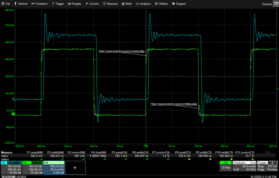
Fig 4 — M4: clean reference. C4: signal after probe loading. C3: waveform via passive probe. Transition differences are clear.
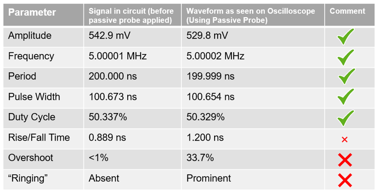
Fig 5 — Comparison between M4 reference and C3 passive probe measurement. Amplitude/frequency agree; transition times do not.
Why Probe Loading Happens
Passive probes carry resistance, capacitance, and inductance in the ground lead. The oscilloscope’s high‑impedance input adds its own resistive and capacitive elements.
Together, they form an RLC network — probe loading — causing overshoot, undershoot, and ringing in captured waveforms.
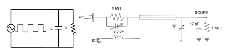
Fig 6 — Equivalent RLC circuit formed when a passive probe connects to a live test point. Combined impedances create probe loading.
High‑impedance inputs are unavoidable with passive probes. Recognizing this mechanism is key to interpreting oscilloscope captures correctly and choosing the right probing method for high‑frequency or signal‑integrity‑critical work.